Edge Detections

So far we have discussed some basics and we know how convolution in image processing works. It is time to talk more about applications of convolution (kernel convolution). So in this post, we will go through Edge Detection algorithms and after reading this post you should be able to understand edge detection concept and its usage in image processing.

Edge Detection

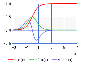
As we know an image is a function of spatial location and values i.e. there is a sort of mapping between location (x, y) and values (3 values for RGB or one value in grayscale images). By considering image definition, we can now define the edges in an image and basically, there are different definition for it (you can find some of them here), but in a nutshell an edge could be defined as points in an image where there are discontinuities or sharp/rapid changes in intensity/values. We can model/estimate these rapid changes as a sigmoid function for each direction by taking derivative of the nearby pixels of the image and when rapid change happens, it can be an edge (this derivative is basically the slope of the line between the points). As shown in Fig. 1, by getting derivative of sigmoid (red curve) function the result is bell shape (green curve) function which shows if we walk on this graph the change in value starts slowly and has a high peak on the edge and again settles down.

Color Spectrum — Fig. 1: Sigmoid function with its 1st & 2nd derivative

Consider that for smoothing the image (noise reduction), as mentioned in last post, we convolve the image with Gaussian kernel and for finding the edges we use convolution of the image with some other kernel. As mentioned before, there are different algorithms to detect the edges in an image which we will discuss some of them here. But before discussing them we should first define Gradient.

Gradient

As we may know from mathematics, Gradient shows the directional changes in a function which is a vector of partial derivative:

$\nabla f = \begin{pmatrix} \frac{\partial f}{\partial x} \ \frac{\partial f}{\partial y} \end{pmatrix} = \frac{\partial f}{\partial x} \vec{i} + \frac{\partial f}{\partial y} \vec{j}$

Roughly said, if we go in gradient direction, then we will reach either local maximum or a local minimum of the function and are corresponds to gradient ascent or descent. In the context of image processing, it points to the pixel which has lower or higher intensity/value.

Edge detection using Sobel Filter (GoG)

Now that we know what are gradient and gaussian, let’s mix them and see what’s happening. Usually, images contain noises (from different sources like sensors) and these noises may cause high gradient in these points and consequently they will be considered as edges. To prevent this problem before applying any edge detection algorithms to the image we should apply the Gaussian filter to smoothe the image. But how do we apply derivative (gradient) to an image? Again we use the definition of derivative for discrete function:

$f'(a) = \lim_{h\to 0}\frac{f(a+h)-f(a)}{h}$

and we will consider h = 1 (each step is one pixel). We can define a kernel that does both steps (smoothing the image and make a derivative in a direction of image) and is called Sobel filter. In another word, it is Gradient of Gaussian. The gradient of Gaussian is one way to find edges in an image for two directions. Fig. 2 shows a Sobel filter (a) for horizontal and (b) vertical edges.

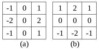
It is important to know that for just getting derivative of the image in x or y directions, we can use Sobel filter and but we should change -2 to -1 and 2 to 1.

To calculate the magnitude and Orientation of the edge, we use the following formulas:

Magnitude (total gradient): $G = \sqrt{G_{x}^2 + G_{y}^2}$ or approx. $G = |G_{x}| + |G_{y}|$
Orientation: $\arctan(\frac{G_{y}}{G_{x}})$

As we can see in the Sobel kernel, the middle row/column are zero and this is because we want to know if the pixel (corresponds to the center of Sobel kernel) is an edge, so if the sum of multiplication of each cell of Sobel kernel and pixel value has high value (magnitude), so the pixel in edge and there is a sharp change in value/intensity of the pixels before and after of the edge. Also in this calculation, the edge value does not have any effect on the result.

Sobel filter is a non-linear filter and can not be replaced by one kernel, so to achieve a proper result we should calculate the magnitude and orientation. Also, it is an approximation of the first derivative and for 3×3 kernel, it is better to use Scharr function in OpenCV.

It should be considered that the direction of the gradient is orthogonal to the edge.

Edge detection using Laplacian (LoG)

Background: Image is a spatial function/domain and each pixel corresponds to a to point(s) in real-world (this called Bijective) with some transformation which is a linear isometry. And the Laplacian operation is an isotropic operator/measure of the second derivative of spatial domain because it is invariant under this linear isometry (transformation) and we can use it.

Another way to detect the edges in an image is Laplacian of Gaussian. We want to find edges when the gradient is very high or very low (by this assumption that sharp changes are a sigmoid function). For that, we can use 2nd derivate of the function and where the second derivative cross the zero means there is a peak in the gradient. To calculate the second derivative we can use the following function:

$f''(x) = \lim_{h\to 0}\frac{f(x+h)-2f(x)+f(x-h)}{h^2}$

We will use the second derivative of the function in both directions (x and y) and Laplacian is the sum of the 2nd partial derivative with respect to x and y.

$\Delta f = \frac{\delta^2f}{\delta x^2} + \frac{\delta^2f}{\delta y^2}$

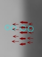
It means we consider a circle and move it around the picture and where the edge is gradient points toward largest change and Laplacian will measure the gradient flowing into the circle and coming out of the circle, see Fig. 3. So near to the edges we have positive/negative value for laplacian and on the center of the edge laplacian would be zero and on the other side of the edge laplacian would be negative/positive and so we consider this part of the image as an edge (it basically measure the divergence of the gradient which is the flux of gradient vector field through small area). The gradient points toward white (255, higher number).

As we go toward this edge the second derivative gets very high and then crosses 0 and goes negative and then goes back to 0, so basically by laplacian on edges we are walking on 2nd derivative of sigmoid, which is shown in Fig. 1 (blue curve), and what important is where it crosses 0. Fig. 4 shows an example of the Laplacian of Gaussian.

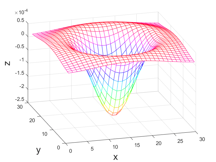
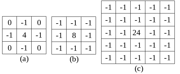
The advantage of Laplacian over Sobel kernel is that it will calculate the total gradient of the image, but it has also a disadvantage which Laplacian is too sensitive to noise and so we always do Laplacian of Gaussian (LoG) which gives a good estimation of edge using 5×5 or 9×9 kernel and on following image you can see three of them.

Edge detection using Fourier Transformation

Fourier Transformation decomposes the function with the sum of sins and cosines which can be divided into high-frequency oscillations and low-frequency oscillations. Basically we are converting image from spatial domain to Fourier domain (Frequency domain).

Discrete Fourier Transform (DFT): $F(k,l) = \sum_{a=0}^{N-1}\sum_{b=0}^{N-1}f(a,b) e^{-i2\pi(\frac{ka}{N}+\frac{lb}{N})}$
Inverse Discrete Fourier Transform: $f(a,b) = \frac{1}{N^2} \sum_{k=0}^{N-1}\sum_{l=0}^{N-1} F(k,l)e^{i2\pi(\frac{ka}{N}+\frac{lb}{N})}$
$e^{ix} = cosx + i sinx$

Where the image is NxN pixels. As we know the edges are high-frequency changes in the image. Consider a basic idea of the High Frequency of an event “A”. If “A” has high frequency then it changes very fast i.e. it has rapid transitions over a given time interval (which in an image it has a rapid transition in the spatial domain). Different edges will be different frequencies depending on how wide they are, For instance, changing color would be low frequencies and very detail in the image would be high frequencies.

So for detecting the edges in an image we can get the DFT of the image and use some sort of high pass filter and apply inverse DFT.

Difference of Gaussian (DoG)

Gaussian is basically a low pass filter which means it goes through the image and removes all fast changes (high frequencies) such as edges, it strongly reduces components with frequency f < f0. So the idea here is to apply a gaussian filter to the image and subtract that with the original image, so the rest would be high-frequency components (edges). We can also use Gaussian filter with high and low frequencies and then subtract them in order to get the components between those frequencies:

$(g(f0) * I)$ -> convolution of Gaussian with high frequency (f0) and original image (I)
$(g(f1) * I)$ -> convolution of Gaussian with low frequency (f1) and original image (I)
components in between f0 and f1: $[g(f0) * I - g(f1) * I] = [g(f0) - g(f1)] * I$

If we subtract the Gaussian functions of different frequencies what we get is a function similar (not same) to the Laplacian of Gaussian and they are doing the same.

Canny Edge Detection

Another way of detecting edges in an image is the Canny algorithm. It is the first image processing pipeline and its algorithm divided into 5 steps:

Smoothing image (only want real edges, not noises) by applying Gaussian filter
Apply Sobel filter to get gradient direction and magnitude. As we know it gives two results (horizontal and vertical edges).
Non-maximum suppression (or gradient) is perpendicular to the edge. Basically what it does is eliminating the repeated detections from the image using considering the maximum probability(confidence) of detected object among others(actually, it gets the value of the neighboring pixels which are along with gradient and see if the value is higher (white) or lower(black) and if it is higher it will select this pixel as an edge).
Threshold into strong, weak, no edge. All of the strong edges are bigger than the threshold. Points are considered as weak edges that are connected to the strong edges (looking at 8 neighborhood pixels).
Connect the components together to form the edges

Sigma(for smoothing) and thresholds are tunable parameters for canny edge detection. Higher sigmas are going to filter out higher frequency information, so by lower sigma, we basically have some sort of detail about edges also some noise too, you can find more about canny algorithm here.

Summary

As we discussed in this post there are different ways for detecting the edges each of which has advantages and disadvantages for instance Laplacian kernel is sensitive to noise but is faster and calculates the total gradient. An important point to mention is that the Gradient of Gaussian results horizontal and vertical edges and the gradient vector is perpendicular to the edge.

Tags:Canny Edge Detection, Computer Vision, Edge Detection, Image Processing, low-level Computer Vision, Machine Learning

About The Author

Tech Enthusiast