Computer Vision Basics

As you may know, demand on Computer Vision Applications is increasing and so I decided to make post series about that and dive into my favorite topic “Computer Vision” and share my knowledge with you to help you to get deep understanding of different topics in this field. These series divided into three parts each of which corresponds to one level of CV. Generally, computer vision topics divided into three levels:

• Low-Level CV in which I will talk about basics of CV as well as its usage in higher level. Low-Level CV mostly consists of working with pixels, image correction, edge detection, feature extraction, etc. Also, in this part, I try to give you some intuition about some functions/basics we use in image processing.
• In Mid-Level CV I will talk about some algorithms used for making a panorama, stereo images, precise feature extraction (RANSAC), optical flow, etc.
• In High-Level CV I will show you how it is possible to leverage machine learning algorithms in CV, so we can do some cool stuff like image classification, detection and so on.

In this post, I will introduce some basic terms and intuitions which can be useful for those of you who do not have any prior knowledge about image processing. After reading this post you know basic definitions that are often used in the context of CV. So Let’s get started.

Low-level Computer Vision

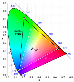
Whenever we take a photo with our camera or smartphone, what we are basically doing is capturing the representation of our environment in the digital world i.e. photo. As shown in Fig. 1 there is a visible color spectrum which we can see in the world but when it comes to computers (digital world) we can just represent/work with a smaller spectrum like sRGB, Adobe RGB, etc.

In a nutshell, cameras are using some sort of Bayer pattern/filter/sensor for identifying the color and convert it to RGB, so the result would an image which can be used in different computers and applications. We can consider this process as some sort of sampling from an analog lightwave. Therefore, all we will do later on images would be working with the RGB value of each pixel. In the following sections, I will describe some basic terms/functions and try to give you some intuition about them, and step by step the more advanced topic will be described.

Some basics

Tensor often you may hear about Tensor but what is that? Roughly said, it is like a matrix to be more precise matrix, which we are using in an engineering context, is a scalar tensor. Basically, tensor is related to vector space which can have different forms. In the context of image processing, it can be used for storing real and complex vectors, color or gray images, etc.

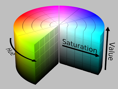
HSV sometimes we need to change our “color model” from RGB to HSV, but what is that? HSV stands for Hue, Saturation, Value. Basically, it is a mechanism to change/set the characteristics of a pixel. Fig. 2 represent the HSV Color model in cylinder model. We can think of HSV as following:

• Hue will determine the base color of the image
• Saturation will determine the intensity of the color compared to white
• Value will determine the brightness of the pixel compared to black

Discrete Fourier Transformation

As you probably know, we can break a function/signal into a sum of sines and cosines of its frequency range which is called Fourier Transform and DFT is just sampled of that. What we will do next is probably filtering some frequencies. In most image processing applications, DFT will be used, but what happens when we apply DFT to an image? how does it make sense? As mentioned before, pixels are a kind of sampled value from analog lightwave so it makes sense to the get DFT of signals and does some filtering on an image in order to remove noise or some frequencies. Now DFT on an image does make sense. We will talk about it later.

Interpolation

As you may know interpolation is used in mathematics, more precise in numerical analysis, as a method for constructing/adding new data points within the range of data. The same concept applies here that means we can use interpolation for resizing, rotating, etc. the images in which we construct a value for a pixel i.e. pixel interpolation.

How to determine the pixel value? To determine the pixel value, there are different interpolation algorithms among which the following ones are mostly used in image processing:

• Nearest neighbor interpolation, as the name says, the pixel value would be same as the value of the nearest pixel. The advantage of this method is the ease of implementation, so it is commonly used in real-time 3D rendering. On the other hand, the result looks blocky and the reason could be integer division as well as rounds down (in C language).

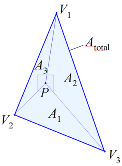
• Triangle interpolation, it considers three pixels around the pixel that we want to interpolate and calculate the value for that with respect to the other three. It used for random sampling of points and roughly say, it calculate the weighted sum of triangular inside the main triangle, as shown in Fig. 3, and normalize it with total area. More detail calculation about the algorithm can be found here.

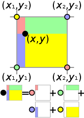
• Bilinear interpolation is a non-linear interpolation which basically is the product of linear interpolation in two dimensions namely X and Y (Height and Width of the image plane), so the process will be divided into two steps: 1) interpolation in both directions 2) interpolation between points results from first step which can use weighted sum based on area of opposite rectangle which shown in Fig. 4. The disadvantage of this interpolation is creating some sort of star-shape pattern (artifacts) where we apply bilinear interpolation.

• Bicubic interpolation is like cubic interpolation but it interpolates data in two dimensions namely X and Y (Height and Width of the image plane) and it considers 16 nearest neighbor pixel for its calculation, therefore, the result is smoother than bilinear, triangle, and nearest-neighbor interpolation, i.e. there would be no star-like pattern. On the other hand, hence, bilinear interpolation uses 4 nearest neighbor pixel for its calculations, it would be faster than bicubic, so bilinear interpolation is a better choice for time-sensitive applications.

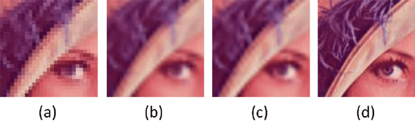
In the following Figure (Fig. 5), we can see the difference between three interpolations, (a) Nearest Neighbor, (b) Bilinear, (c) Bicubic and (c) original.

That’s it for this post, I hope you enjoyed it and leave a comment if you have any suggestion/request/question about computer vision series. In the next post, I will dive deeper into the low-level CV.